
Study on Toronto's bicycle thefts
- Leonardo Patricelli
- Sep 25, 2020
- 4 min read
Updated: Sep 26, 2020
Hello Toronto!
My bike got stolen recently, so I decided to go deeper into this the only way I know, with statistics. Moreover, I wanted to try an XGBoost model with R. So here I am.
I will not discuss in here the math and the code used to generate this info, but I'll post an attachment with the R script I wrote with my notes. The package used for data visualization is Ggplot2.
1. Getting ready
First of all, let's download the data from Toronto's open data portal. Here is the link:
This website posts a lot of free datasets about the city of Toronto. Most of the data are police records and, usually, all the data have a field containing the neighbourhood. In this website, I found data about byke thefts from 2014 to 2019. Here is the link with all the details.
From the Toronto open data website, you can also download the city shapefile (a kind of map that you can use to plot statistics). Here is the link.
The most important features used in this analysis are:
The date on which the theft occurred;
The neighborhood of the theft.
It could be really interesting and useful to use the information about the bike model contained in the dataset, but the variables have a serious problem with consistency. In fact, there is no info about the labels used and there are too many missing values to use the variable in the analysis.
Let's start our exploratory analysis.
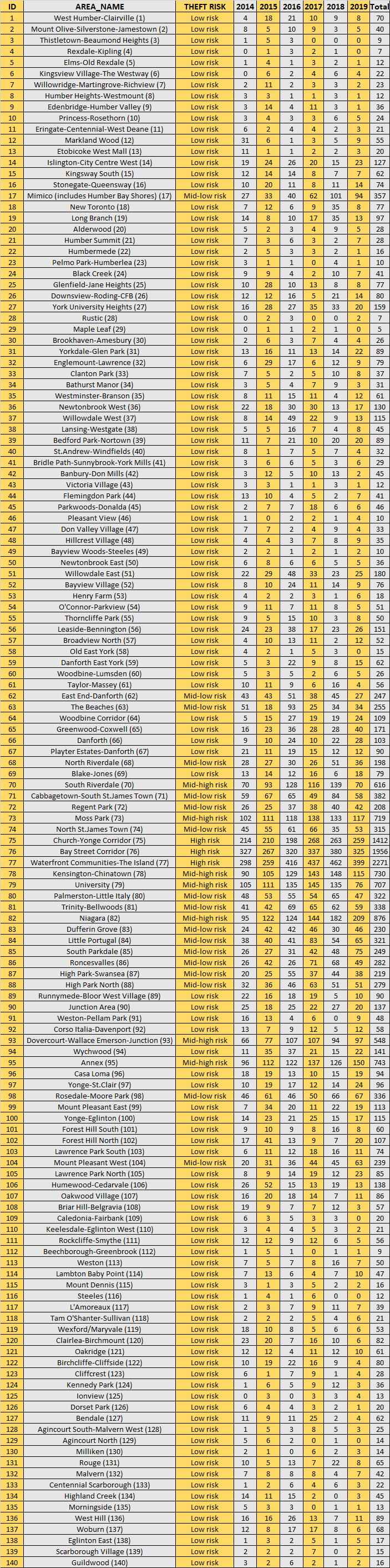
The map below shows Toronto's neighborhoods. Inside each neighborhood, I wrote the relative ID number. The table below shows the names.

Here it is a brief description :
ID is the ID number displayed in the map above;
Area_name is the name of the neighborhood;
Theft Risk is divided into 4 categories, fro low risk to high risk, and determines the chance of theft;
The year says the number of thefts occurred that year in a specific neighborhood;
Total is the total of bike stolen in a neighborhood in the latest 6 years.
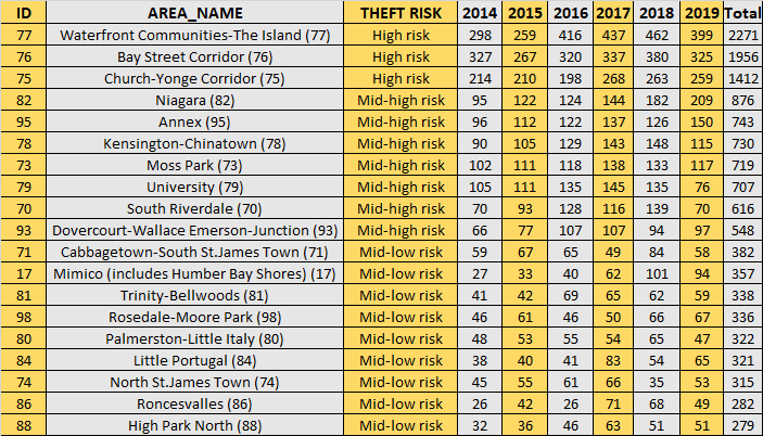
2. Top 20 neighborhoods
In this table, the neighborhoods are sorted in descending order of the number of stolen bikes.
The majority of thefts happen downtown, in the entertainment district and close to Yonge-Dundas Square. In addition, it seems that the more you move away from these zones, the more the number of thefts decreases.
Neighborhoods close to the entertainment district have a mid-high risk associated, while further neighborhoods just low or mid-low.
3. Exploratory analysis
Let's start plotting the distribution of the thefts in each month. Maybe you didn't know it, but Toronto is really cold in the winter, so I think they are more likely to happen in summer rather than in winter.
Let's have a look. In each bar, I wrote the number of thefts that occurred during the relative month.
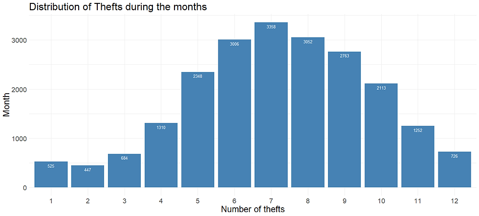
It seems that the thefts have a normal distribution and that most crimes happen during the summer (when it's hot and people are more likely to go out with their own bike for a ride). The number on top of the bar is the number of thefts that occurred during that specific hour in the last 6 years.

The graph of the hourly distribution shows that most thefts happen in the evening.
Let's have a look at the number of thefts per neighborhood from 2014 to 2019. I wrote the number of thefts that occurred each year in each neighborhood area. Click on the images to zoom.
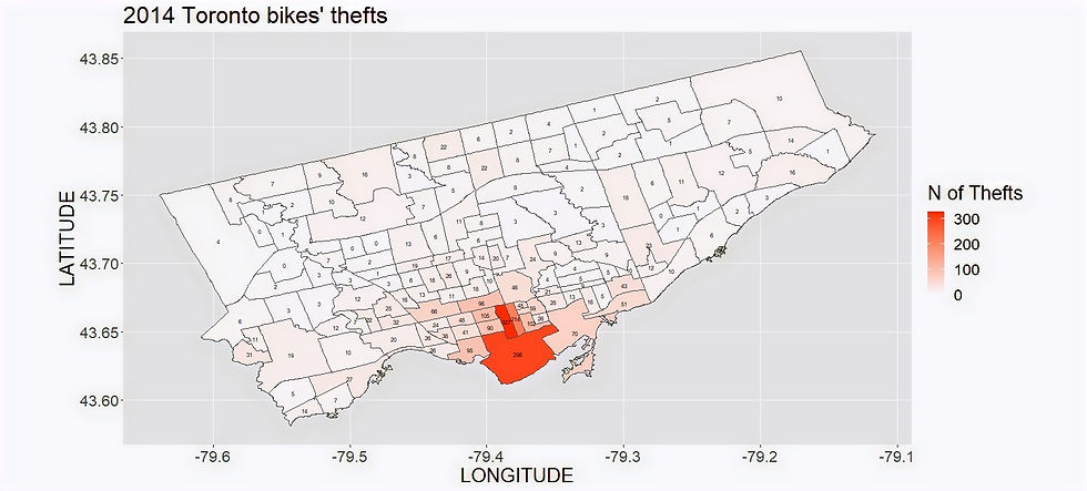
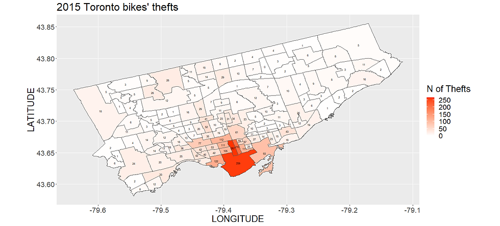

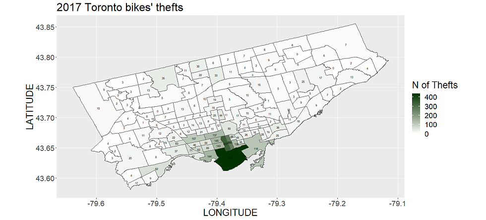
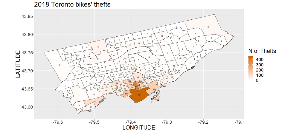

You can notice that most of them happen downtown and in the university/campus area. So if you leave your bike there, watch out!
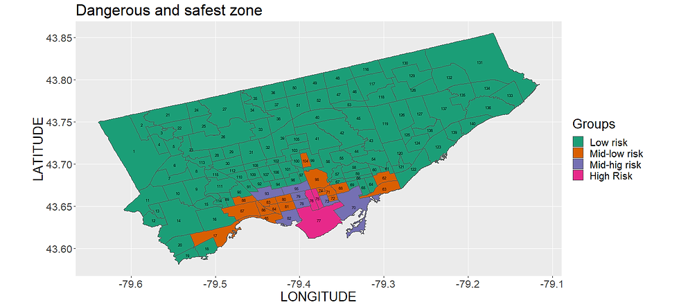
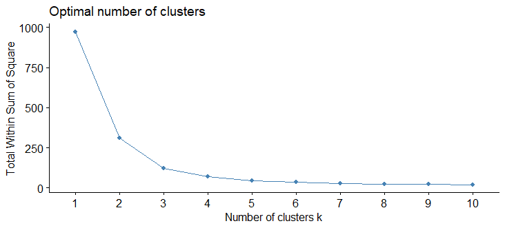
4. Clustering
We can notice that there are areas in which thefts happen more frequently. We can create categories according to the number of thefts per year.
To do so we are going to use an unsupervised machine learning method called "hierarchical clustering". The elbow method shows us the optimal number of clusters is 4.
Here are the results.
5. XGBoost model predictions
Now let's try to predict the number of thefts that will happen in summer 2019. Unfortunately, we don't have 2020 data, so we cannot predict them. in addition, due to COVID-19, the number of riders around the town will be way less than before, so it means also fewer thefts.
Let's see the performance of the model.
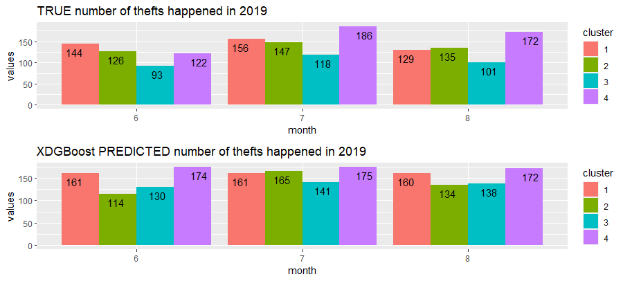
Here let's compare the prediction with the true values.
In the last row of each table you can notice the difference in percentage.
When the number is positive, it means the model is overestimating the thefts, viceversa if negative it is underestimating. In the bottom right cell there is the total comparison.

June has a high bias in estimations (almost 20%), while July has only a 7% error rate.
The overall model performance is not so great, with an error rate of 12.03 %.
To improve this result we could use some feature engineering and add, for example, a variable for the season or related to the major crimes (there is a dataset on the Toronto open data portal about it), but we are not going to do that.
Hope you enjoyed it! And watch out your bike!
Leonardo,
The pizza Statistician
P.s. Here you can download the script
Comments